House Prices: Advanced Regression Techniques

프로젝트 명: 집값예측-심화 (House Prices: Advanced Regression Techniques)

본 프로젝트는 주어진 집(house) 관련 데이터를 토대로 집 값을 예측하는 회귀(Regression) 분석 및 예측 대회입니다.

데이터 출처: House Prices: Advanced Regression Techniques

프로젝트 개요

[원문]

Ask a home buyer to describe their dream house, and they probably won’t begin with the height of the basement ceiling or the proximity to an east-west railroad. But this playground competition’s dataset proves that much more influences price negotiations than the number of bedrooms or a white-picket fence.

With 79 explanatory variables describing (almost) every aspect of residential homes in Ames, Iowa, this competition challenges you to predict the final price of each home.

[번역]

집 구매자에게 꿈의 집을 묘사해달라고 물어본다면, 그들은 지하실 천장 높이나 ‘동서(east-west) 철도와의 근접성’이라고 대답하지는 않을 것입니다. 그런데 본 데이터 세트는 앞서 얘기한 요소들이 침실 수 또는 하얀 울타리보다 가격 협상에 훨씬 더 많은 영향을 준다는 것을 알 수 있게됩니다.

본 프로젝트는 79개의 다양한 집을 묘사할 수 있는 데이터 요소들을 기반으로, 각각의 집들에 대하여 최종 집값을 예측해 주길 기대합니다.

지금 까지 배운 모든 내용을 집대성하여, 집 값 예측에 도전합니다.

프로젝트 목표

1. '섬세한' 데이터 전처리와 창의적인 feature engineering
2. 데이터 시각화를 통한 데이터 특성을 파악합니다.
3. `pandas`, `numpy`, `scikit-learn` 패키지를 활용하여 데이터 병합, 전처리, 피처 공학(feature engineering)을 진행합니다.
4. 회귀문제를 다루는 고급 머신러닝 기법을 활용하여 주택 가격 예측을 진행합니다.
4. 회귀 모델과 다양한 모델들 간의 앙상블 학습을 통해 모델의 성능을 끌어올립니다.

프로젝트 구성

* 데이터 로드 (load data)
* 데이터 시각화 (visualization)
* 데이터 전처리 (pre-processing)
* 머신러닝을 활용하여 baseline 모델링 (modeling for baseline)
* 평가지표 생성 (evalutation)
* 모델 앙상블, 데이터 전처리 개선으로 모델의 성능을 업그레이드 하여, 목표 점수에 도달

팁

다음의 기술 및 분석 능력을 통해 보다 정확한 예측 성능(performance)을 기대할 수 있습니다.

* 데이터 전처리 (preprocessing)를 통하여, 결측치(NaN), 극단치(outlier) 처리
* 데이터 시각화 (EDA - Exploratory Data Analysis, 탐색적 데이터 분석)
* 데이터에는 결측치도 굉장히 많이 존재하고, 이상치(outlier)도 존재합니다. 실전 데이터를 통해 이를 잘 처리해 주어야먄 좋은 점수를 기대할 수 있습니다.
* 다양한 모델들의 앙상블을 통해 획기적인 점수 개선을 눈으로 직접 확인할 수 있습니다. 좋은 모델을 선정하고, baggine, boosting, stacking 등의 앙상블 기법을 통해 점수 개선을 기대해 봅니다.

• 작성자: 이경록 감수자

---

데이터

아래 링크를 통해 데이터를 다운로드 받을 수 있습니다.

• train.csv
• test.csv
• submission.csv

데이터 column에 대한 설명입니다.

• SalePrice - 집 값 (우리가 예측 해야할 가격)
• MSSubClass: The building class
• MSZoning: The general zoning classification
• LotFrontage: Linear feet of street connected to property
• LotArea: Lot size in square feet
• Street: Type of road access
• Alley: Type of alley access
• LotShape: General shape of property
• LandContour: Flatness of the property
• Utilities: Type of utilities available
• LotConfig: Lot configuration
• LandSlope: Slope of property
• Neighborhood: Physical locations within Ames city limits
• Condition1: Proximity to main road or railroad
• Condition2: Proximity to main road or railroad (if a second is present)
• BldgType: Type of dwelling
• HouseStyle: Style of dwelling
• OverallQual: Overall material and finish quality
• OverallCond: Overall condition rating
• YearBuilt: Original construction date
• YearRemodAdd: Remodel date
• RoofStyle: Type of roof
• RoofMatl: Roof material
• Exterior1st: Exterior covering on house
• Exterior2nd: Exterior covering on house (if more than one material)
• MasVnrType: Masonry veneer type
• MasVnrArea: Masonry veneer area in square feet
• ExterQual: Exterior material quality
• ExterCond: Present condition of the material on the exterior
• Foundation: Type of foundation
• BsmtQual: Height of the basement
• BsmtCond: General condition of the basement
• BsmtExposure: Walkout or garden level basement walls
• BsmtFinType1: Quality of basement finished area
• BsmtFinSF1: Type 1 finished square feet
• BsmtFinType2: Quality of second finished area (if present)
• BsmtFinSF2: Type 2 finished square feet
• BsmtUnfSF: Unfinished square feet of basement area
• TotalBsmtSF: Total square feet of basement area
• Heating: Type of heating
• HeatingQC: Heating quality and condition
• CentralAir: Central air conditioning
• Electrical: Electrical system
• 1stFlrSF: First Floor square feet
• 2ndFlrSF: Second floor square feet
• LowQualFinSF: Low quality finished square feet (all floors)
• GrLivArea: Above grade (ground) living area square feet
• BsmtFullBath: Basement full bathrooms
• BsmtHalfBath: Basement half bathrooms
• FullBath: Full bathrooms above grade
• HalfBath: Half baths above grade
• Bedroom: Number of bedrooms above basement level
• Kitchen: Number of kitchens
• KitchenQual: Kitchen quality
• TotRmsAbvGrd: Total rooms above grade (does not include bathrooms)
• Functional: Home functionality rating
• Fireplaces: Number of fireplaces
• FireplaceQu: Fireplace quality
• GarageType: Garage location
• GarageYrBlt: Year garage was built
• GarageFinish: Interior finish of the garage
• GarageCars: Size of garage in car capacity
• GarageArea: Size of garage in square feet
• GarageQual: Garage quality
• GarageCond: Garage condition
• PavedDrive: Paved driveway
• WoodDeckSF: Wood deck area in square feet
• OpenPorchSF: Open porch area in square feet
• EnclosedPorch: Enclosed porch area in square feet
• 3SsnPorch: Three season porch area in square feet
• ScreenPorch: Screen porch area in square feet
• PoolArea: Pool area in square feet
• PoolQC: Pool quality
• Fence: Fence quality
• MiscFeature: Miscellaneous feature not covered in other categories
• MiscVal: $Value of miscellaneous feature
• MoSold: Month Sold
• YrSold: Year Sold
• SaleType: Type of sale
• SaleCondition: Condition of sale

필요한 라이브러리와 데이터를 import 합니다.

import pandas as pd
import numpy as np
import matplotlib.pyplot as plt
import warnings
import seaborn as sns
import os

warnings.filterwarnings('ignore')
%matplotlib inline

데이터를 불러옵니다.

• train: 학습에 필요한 데이터
• test: 예측을 위한 데이터

train = pd.read_csv('https://bit.ly/fc-ml-byte-final-train')
test = pd.read_csv('https://bit.ly/fc-ml-byte-final-test')

train.shape, test.shape

((1460, 81), (1459, 80))

tip shape를 보니, train 데이터와 test 데이터의 행의 갯수가 거의 동일합니다.

1. train set가 많을 때는 어느 정도 학습을 충분히 시켜줘야합니다.
2. 하지만, 이렇게 데이터 행의 갯수가 비슷할 때는 과적합이 되지 않도록, 유의해야합니다.

예측 값 - SalePrice

우리가 예측해야할 label: SalePrice 입니다.

SalePrice는 주택 가격을 의미합니다.

train['SalePrice'].head()

0    208500
1    181500
2    223500
3    140000
4    250000
Name: SalePrice, dtype: int64

예측 값 (SalePrice) 에 대한 탐색적 데이터 분석

train 데이터 셋에만 SalePrice가 존재 합니다.

예측 값에 대한 간단한 통계 지표를 확인해 보겠습니다.

train['SalePrice'].describe()

count      1460.000000
mean     180921.195890
std       79442.502883
min       34900.000000
25%      129975.000000
50%      163000.000000
75%      214000.000000
max      755000.000000
Name: SalePrice, dtype: float64

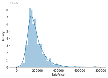
Q1. distplot으로 우리가 예측할 SalePrice column에 대한 가격 분포를 확인해 주세요

# 코드를 입력하세요
sns.distplot(train['SalePrice']);

label 생성

label = train['SalePrice']

train = train.drop('SalePrice', 1)

전처리: 데이터 합치기

보다 효율적인 데이터 전처리를 위해서 train 데이터프레임과 test 데이터프레임을 모두 합쳐서 한꺼번에 전처리 해주는 것을 추천드립니다.

Q2. all_data 변수를 만들고 train + test 데이터프레임을 합쳐 주세요 (concat)

1. id column은 단순한 순번이므로, column에서 drop 합니다.
2. all_data란느 변수에 train과 test 데이터프레임을 합침니다.
3. index를 reset 합니다.

train = train.drop('Id', 1)
test = test.drop('Id', 1)

# 코드를 입력해 주세요
all_data = pd.concat([train, test], sort=False, ignore_index=True)

# 검증코드
print('테스트 결과: {}'.format(all_data.shape == (2919, 79)))

# 결과 출력
print(all_data.shape)
all_data.head()

테스트 결과: True
(2919, 79)

	MSSubClass	MSZoning	LotFrontage	LotArea	Street	Alley	LotShape	LandContour	Utilities	LotConfig	...	ScreenPorch	PoolArea	PoolQC	Fence	MiscFeature	MiscVal	MoSold	YrSold	SaleType	SaleCondition
0	60	RL	65.0	8450	Pave	NaN	Reg	Lvl	AllPub	Inside	...	0	0	NaN	NaN	NaN	0	2	2008	WD	Normal
1	20	RL	80.0	9600	Pave	NaN	Reg	Lvl	AllPub	FR2	...	0	0	NaN	NaN	NaN	0	5	2007	WD	Normal
2	60	RL	68.0	11250	Pave	NaN	IR1	Lvl	AllPub	Inside	...	0	0	NaN	NaN	NaN	0	9	2008	WD	Normal
3	70	RL	60.0	9550	Pave	NaN	IR1	Lvl	AllPub	Corner	...	0	0	NaN	NaN	NaN	0	2	2006	WD	Abnorml
4	60	RL	84.0	14260	Pave	NaN	IR1	Lvl	AllPub	FR2	...	0	0	NaN	NaN	NaN	0	12	2008	WD	Normal

5 rows × 79 columns

전처리: NaN 값 채우기

Q3. NaN 값을 포함하는 column과 NaN 값의 갯수를 출력합니다.

missing 이라는 데이터프레임에 NaN 값을 포함하는 column과 NaN 값의 갯수 정보를 담습니다.

# 코드를 입력하세요 #
missing = all_data.isnull().sum()

#####################
missing.sort_values(ascending=False).head()

PoolQC         2909
MiscFeature    2814
Alley          2721
Fence          2348
FireplaceQu    1420
dtype: int64

Q4. LotFrontage 에 대한 NaN값 (결측치) 채워주기

LotFrontage에 대한 NaN값을 채워 주도록 하겠습니다.

• Neighborhood column, 즉 같은 이웃간에는 비슷한 크기의 LotFrontage를 가진다라는 전제하겠습니다.
• 빈 값을 채워줄 때 groupby 메소드를 활용하여 같은 Neighborhood 끼리의 LotFrontage 중앙값(median) 으로 채워주도록 합니다.

all_data_backup = all_data.copy()

# 코드를 입력하세요
LotFrontage_median = all_data.groupby('Neighborhood')['LotFrontage'] \
            .agg(['median'])
LotFrontage_median.head(10)

	median
Neighborhood
Blmngtn	43.0
Blueste	24.0
BrDale	21.0
BrkSide	51.0
ClearCr	80.5
CollgCr	70.0
Crawfor	70.0
Edwards	65.0
Gilbert	64.0
IDOTRR	60.0

all_data[:10][['LotFrontage', 'Neighborhood']]

	LotFrontage	Neighborhood
0	65.0	CollgCr
1	80.0	Veenker
2	68.0	CollgCr
3	60.0	Crawfor
4	84.0	NoRidge
5	85.0	Mitchel
6	75.0	Somerst
7	NaN	NWAmes
8	51.0	OldTown
9	50.0	BrkSide

all_data["LotFrontage"] = all_data.groupby(["Neighborhood"])["LotFrontage"].transform(lambda x: x.fillna(x.median()))

# 정답 체크용 함수
def check_pass(df):
    assert df['LotFrontage'][7] == 80.0
    assert df['LotFrontage'][100] == 80.0
    assert df['LotFrontage'][166] == 80.5
    assert df['LotFrontage'][2727] == 73.0
    assert df['LotFrontage'][2839] == 70.0
    assert df['LotFrontage'].isnull().sum() == 0
    print('통과~')
    
check_pass(all_data)

통과~

잘못된 데이터 수정하기

all_data['PoolQC'].isnull().sum()

2909

가끔은 잘못된 데이터가 들어가 있는 경우가 있습니다. 이럴 땐 상식적으로 맞는 값으로 다시 수정해 줄 필요가 있습니다.

잘못된 값을 수정해 주세요

(hint) GarageYrBlt

all_data['GarageYrBlt'].sort_values(ascending=False).head()

2592    2207.0
378     2010.0
1608    2010.0
819     2010.0
987     2010.0
Name: GarageYrBlt, dtype: float64

all_data.loc[all_data['GarageYrBlt'] == 2207, 'GarageYrBlt'] = 2007

NaN 값이 포함된 column은 다음 2가지 방법으로 처리할 수 있습니다.

1. 적절한 값으로 채워준다
2. 아예 column 자체를 drop 하여 사용하지 않는다.

일단, 우리는 1번 방법인 적절한 값으로 채워주도록 하겠습니다.

전처리: 숫자형/문자형 column별 NaN 값 채우기

Q5. 수치형 (numerical) 컬럼과 카테고리형 (categorical) 컬럼 나누기

먼저, 숫자형으로 이루어진 column과 문자형으로 이루어진 column을 구분해 주도록 하겠습니다.

# LotFrontage NaN값 (결측치) 처리 이후 바뀌었으므로 다시 받음
missing = all_data.isnull().sum()

missing = missing[missing > 0]

nan_cols = missing.keys()

all_data[nan_cols].isnull().sum()

MSZoning           4
Alley           2721
Utilities          2
Exterior1st        1
Exterior2nd        1
MasVnrType        24
MasVnrArea        23
BsmtQual          81
BsmtCond          82
BsmtExposure      82
BsmtFinType1      79
BsmtFinSF1         1
BsmtFinType2      80
BsmtFinSF2         1
BsmtUnfSF          1
TotalBsmtSF        1
Electrical         1
BsmtFullBath       2
BsmtHalfBath       2
KitchenQual        1
Functional         2
FireplaceQu     1420
GarageType       157
GarageYrBlt      159
GarageFinish     159
GarageCars         1
GarageArea         1
GarageQual       159
GarageCond       159
PoolQC          2909
Fence           2348
MiscFeature     2814
SaleType           1
dtype: int64

일단 수치형 컬럼과 / 카테고리형 컬럼을 나누어 각각 변수에 할당합니다.

• num_cols: NaN 값으로 이루어진 수치형 column
• cat_cols: NaN 값으로 이루어진 문자형 column

hint) select_dtypes

# 이곳에 코드를 입력해 주세요
num_cols = all_data[nan_cols].select_dtypes(exclude = ["object"] ).columns
all_data[num_cols].info()

<class 'pandas.core.frame.DataFrame'>
RangeIndex: 2919 entries, 0 to 2918
Data columns (total 10 columns):
 #   Column        Non-Null Count  Dtype  
---  ------        --------------  -----  
 0   MasVnrArea    2896 non-null   float64
 1   BsmtFinSF1    2918 non-null   float64
 2   BsmtFinSF2    2918 non-null   float64
 3   BsmtUnfSF     2918 non-null   float64
 4   TotalBsmtSF   2918 non-null   float64
 5   BsmtFullBath  2917 non-null   float64
 6   BsmtHalfBath  2917 non-null   float64
 7   GarageYrBlt   2760 non-null   float64
 8   GarageCars    2918 non-null   float64
 9   GarageArea    2918 non-null   float64
dtypes: float64(10)
memory usage: 228.2 KB

cat_cols = all_data[nan_cols].select_dtypes(include = ["object"]).columns
all_data[cat_cols].info()

<class 'pandas.core.frame.DataFrame'>
RangeIndex: 2919 entries, 0 to 2918
Data columns (total 23 columns):
 #   Column        Non-Null Count  Dtype 
---  ------        --------------  ----- 
 0   MSZoning      2915 non-null   object
 1   Alley         198 non-null    object
 2   Utilities     2917 non-null   object
 3   Exterior1st   2918 non-null   object
 4   Exterior2nd   2918 non-null   object
 5   MasVnrType    2895 non-null   object
 6   BsmtQual      2838 non-null   object
 7   BsmtCond      2837 non-null   object
 8   BsmtExposure  2837 non-null   object
 9   BsmtFinType1  2840 non-null   object
 10  BsmtFinType2  2839 non-null   object
 11  Electrical    2918 non-null   object
 12  KitchenQual   2918 non-null   object
 13  Functional    2917 non-null   object
 14  FireplaceQu   1499 non-null   object
 15  GarageType    2762 non-null   object
 16  GarageFinish  2760 non-null   object
 17  GarageQual    2760 non-null   object
 18  GarageCond    2760 non-null   object
 19  PoolQC        10 non-null     object
 20  Fence         571 non-null    object
 21  MiscFeature   105 non-null    object
 22  SaleType      2918 non-null   object
dtypes: object(23)
memory usage: 524.6+ KB

# 검증 코드
# 본 cell 실행시 에러가 나지 않아야 합니다.
# assert len(num_cols) == 11

# 엄밀히 따지면 LotFrontage는 위에서 이미 Neighborhood 끼리의 LotFrontage 중앙값(median) 으로 전처리를 하였기 때문에 num_cols 제외 시킴
assert len(num_cols) == 10
assert len(cat_cols) == 23

Q6. 수치형 (numerical) 컬럼에 대해서는 중앙 값으로 결측치를 채워주겠습니다.

all_data[num_cols]에 대해서는 중앙값(median)으로 값을 채워주도록 하겠습니다.

all_data[num_cols].isnull().sum()

MasVnrArea       23
BsmtFinSF1        1
BsmtFinSF2        1
BsmtUnfSF         1
TotalBsmtSF       1
BsmtFullBath      2
BsmtHalfBath      2
GarageYrBlt     159
GarageCars        1
GarageArea        1
dtype: int64

# 이곳에 코드를 입력해 주세요
all_data[num_cols] = all_data[num_cols].fillna(all_data[num_cols].median())

all_data[num_cols].isnull().sum()

MasVnrArea      0
BsmtFinSF1      0
BsmtFinSF2      0
BsmtUnfSF       0
TotalBsmtSF     0
BsmtFullBath    0
BsmtHalfBath    0
GarageYrBlt     0
GarageCars      0
GarageArea      0
dtype: int64

# 검증코드
assert all_data[num_cols].isnull().sum().sum() == 0

Q7. 카테고리형 (categorical) 컬럼에 대해서는 ‘None’ 으로 결측치를 채워주겠습니다.

all_data[cat_cols]에 대해서는 'None'이라는 문자열 값으로 채워주도록 하겠습니다.

# 이곳에 코드를 입력해 주세요
all_data[cat_cols] = all_data[cat_cols].fillna("None")

all_data[cat_cols].isnull().sum()

MSZoning        0
Alley           0
Utilities       0
Exterior1st     0
Exterior2nd     0
MasVnrType      0
BsmtQual        0
BsmtCond        0
BsmtExposure    0
BsmtFinType1    0
BsmtFinType2    0
Electrical      0
KitchenQual     0
Functional      0
FireplaceQu     0
GarageType      0
GarageFinish    0
GarageQual      0
GarageCond      0
PoolQC          0
Fence           0
MiscFeature     0
SaleType        0
dtype: int64

# 검증코드
# 본 cell을 실행해서 에러가 나지 않아야 합니다.
assert all_data[cat_cols].isnull().sum().sum() == 0

전처리: Outlier 확인 및 제거

plt.figure(figsize=(9, 6))
sns.regplot(x=train['GrLivArea'], y=np.log1p(label))

<AxesSubplot:xlabel='GrLivArea', ylabel='SalePrice'>

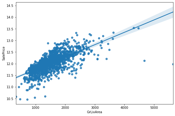
위의 그래프를 보면, 몇 개의 outlier가 보입니다.

데이터의 모수가 작을 수록, 몇 개의 outlier 데이터가 전체 성능에 미치는 영향이 매우 큽니다.

outlier를 확인하고 제거합니다.

제거한 후 변경 후 regplot을 살펴볼까요?

plt.figure(figsize=(9, 6))
sns.regplot(x=train.drop([1298, 523],0)['GrLivArea'], y=np.log1p(label.drop([1298, 523],0)))

<AxesSubplot:xlabel='GrLivArea', ylabel='SalePrice'>

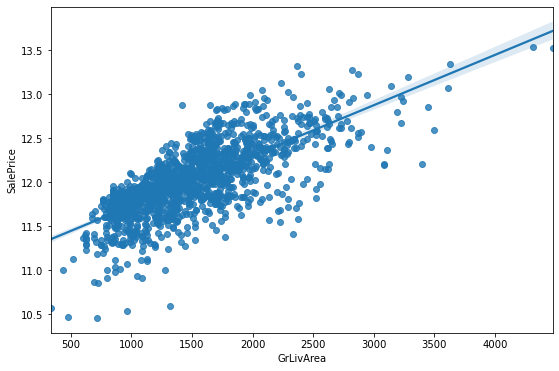
좀 더 깔끔해진 선형 관계를 확인할 수 있습니다.

# 나중에 all_data를 train/ test 데이터 셋으로 분리 후 제거해주도록 하겠습니다.
outlier = [523, 1298]

train.loc[outlier]['GrLivArea']

523     4676
1298    5642
Name: GrLivArea, dtype: int64

Feature Engineering: 새로운 feature 생성

다음 7개의 column은 한마디로 집의 옵션과 같은 개념입니다.

아무래도 옵션이 존재하면 높은 집값의 요인이 될 수 있고, 옵션이 빠진다면, 집값이 비교적 낮겠죠.

0은 옵션이 없다고 해석할 수 있고, 0 이상의 값은 옵션이 존재한다는 의미라고 해석할 수 있습니다.

아래 6개의 column에 대하여 옵션의 존재 유무에 대한 기존의 column은 유지하되, 새로운 column을 만들어 존재하면 1, 없으면 0으로 구성된 column을 새롭게 만들어 주세요

• WoodDeckSF
• OpenPorchSF
• EnclosedPorch
• 3SsnPorch
• ScreenPorch
• PoolArea
• Fireplaces

WoodDeckSF에 대한 샘플 코드를 참고해주세요

Q8. 위에 명시한 7개의 column에 대하여 아래 샘플 코드와 같이 새로운 feature를 생성해 주세요.

# 샘플코드
all_data['WoodDeckSF_bool'] = all_data['WoodDeckSF'].apply(lambda x: 1 if x > 0 else 0)

# 이곳에 코드를 입력해 주세요
all_data['OpenPorchSF_bool'] = all_data['OpenPorchSF'].apply(lambda x: 1 if x > 0 else 0)
all_data['EnclosedPorch_bool'] = all_data['EnclosedPorch'].apply(lambda x: 1 if x > 0 else 0)
all_data['3SsnPorch_bool'] = all_data['3SsnPorch'].apply(lambda x: 1 if x > 0 else 0)
all_data['ScreenPorch_bool'] = all_data['ScreenPorch'].apply(lambda x: 1 if x > 0 else 0)
all_data['PoolArea_bool'] = all_data['PoolArea'].apply(lambda x: 1 if x > 0 else 0)
all_data['Fireplaces_bool'] = all_data['Fireplaces'].apply(lambda x: 1 if x > 0 else 0)

all_data.shape

(2919, 86)

Feature Engineering: 소수 데이터를 다수로 치환

소수 값을 가진 데이터들이 있습니다. 예를 들면, MiscFeature column의 TenC 값은 단 1개의 row 밖에 없습니다.

소수의 값을 가진 데이터들이 존재하면, 전체 트렌드를 파악해야하는 model의 성능을 떨어뜨릴 수 있습니다.

그래서, 소수 데이터를 우리는 다른 다수의 값으로 치환될 수 있도록 하겠습니다.

all_data.loc[all_data['MiscFeature'] == 'TenC']

	MSSubClass	MSZoning	LotFrontage	LotArea	Street	Alley	LotShape	LandContour	Utilities	LotConfig	...	YrSold	SaleType	SaleCondition	WoodDeckSF_bool	OpenPorchSF_bool	EnclosedPorch_bool	3SsnPorch_bool	ScreenPorch_bool	PoolArea_bool	Fireplaces_bool
1386	60	RL	80.0	16692	Pave	None	IR1	Lvl	AllPub	Inside	...	2006	WD	Normal	0	1	0	0	1	1	1

1 rows × 86 columns

None 값이 많은 [‘Alley’, ‘MiscFeature’] 컬럼에 대해서는 값이 None이 아니면 1 None이면 0으로 바꿔주도록 하겠습니다.

all_data['Alley'].value_counts()

None    2721
Grvl     120
Pave      78
Name: Alley, dtype: int64

all_data['MiscFeature'].value_counts()

None    2814
Shed      95
Gar2       5
Othr       4
TenC       1
Name: MiscFeature, dtype: int64

# 샘플코드
all_data['Alley_bool'] = all_data['Alley'].apply(lambda x: 0 if x == 'None' else 1)
all_data['MiscFeature_bool'] = all_data['MiscFeature'].apply(lambda x: 0 if x == 'None' else 1)

Q9. 소수 값을 가진 데이터 바꾸기

그 밖에 소수의 값들로 이루어진 데이터는 새로운 데이터 그룹을 만들어 치환하도록 하겠습니다.

예를 들면, Functional column 에서 Typ가 주를 이루고 있는데, Typ가 아닌 값들은 Other로 바꿔보겠습니다.

all_data['Functional'].value_counts()

Typ     2717
Min2      70
Min1      65
Mod       35
Maj1      19
Maj2       9
Sev        2
None       2
Name: Functional, dtype: int64

위의 샘플 코드를 참고하여, Functional 컬럼의 값이 Typ 이 아닌 값은 Other로 치환해 주세요..

# 코드를 입력해 주세요
all_data['Functional'] = all_data['Functional'].apply(lambda x: 'Typ' if x == 'Typ' else 'Other')

all_data['Functional'].value_counts()

Typ      2717
Other     202
Name: Functional, dtype: int64

# All_data 추적_질의응답_ver2.ipynb 에서 추가 함
all_data['Electrical'] = all_data['Electrical'].apply(lambda x: x if x == 'SBrkr' else 'Fuse')
all_data['RoofMatl'] = all_data['RoofMatl'].apply(lambda x: x if x == 'CompShg' else 'Other')
all_data['GarageQual'] = all_data['GarageQual'].apply(lambda x: x if x == 'TA' else 'Other')
ext_other = [
    'Stone',
    'AsphShn',
    'Other',
    'CBlock',
    'ImStucc',
    'Brk Cmn',
    'BrkComm',
    'None',
]
saletype_other = [
    'ConLD',
    'ConLw',
    'ConLI',
    'CWD',
    'Oth',
    'Con',
    'None'
]

all_data['Exterior1st'] = all_data['Exterior1st'].apply(lambda x: 'Other' if x in ext_other else x)
all_data['Exterior2nd'] = all_data['Exterior2nd'].apply(lambda x: 'Other' if x in ext_other else x)

all_data['SaleType'] = all_data['SaleType'].apply(lambda x: x if x not in saletype_other else 'Other')

Feature Engineering: 새로운 feature 생성 (column 간 연산)

1층 화장실의 갯수와 2층 화장실의 갯수를 더해서 전체 화장실을 구해볼 수 있거나,

구역별 면적을 더해서 전체 집의 면적을 나타내는 column을 생성할 수 있습니다.

Q10-1. total_area

• 새로운 total_area column을 생성하고 [‘BsmtFinSF1’, ‘BsmtFinSF2’, ‘1stFlrSF’, ‘2ndFlrSF’] column의 값을 모두 합산한 값을 대입해 주세요

all_data_backup = all_data.copy

# 이곳에 코드를 입력해 주세요
all_data['total_area'] = all_data['BsmtFinSF1'] + all_data['BsmtFinSF2'] + all_data['1stFlrSF'] + all_data['2ndFlrSF']

all_data[['total_area', 'BsmtFinSF1', 'BsmtFinSF2', '1stFlrSF', '2ndFlrSF']].head()

	total_area	BsmtFinSF1	BsmtFinSF2	1stFlrSF	2ndFlrSF
0	2416.0	706.0	0.0	856	854
1	2240.0	978.0	0.0	1262	0
2	2272.0	486.0	0.0	920	866
3	1933.0	216.0	0.0	961	756
4	2853.0	655.0	0.0	1145	1053

Q10-2. other_area

• WoodDeckSF
• OpenPorchSF
• EnclosedPorch
• 3SsnPorch
• ScreenPorch

컬럼들에 대한 총 면적을 구하는 새로운 other_area 컬럼을 생성해 주세요

# 이곳에 코드를 입력해 주세요
all_data['other_area'] = all_data['WoodDeckSF'] + all_data['OpenPorchSF'] + all_data['EnclosedPorch'] \
                        + all_data['3SsnPorch'] + all_data['ScreenPorch']

all_data[['other_area', 'WoodDeckSF', 'OpenPorchSF', 'EnclosedPorch', '3SsnPorch', 'ScreenPorch']].head()

	other_area	WoodDeckSF	OpenPorchSF	EnclosedPorch	3SsnPorch	ScreenPorch
0	61	0	61	0	0	0
1	298	298	0	0	0	0
2	42	0	42	0	0	0
3	307	0	35	272	0	0
4	276	192	84	0	0	0

Q10-3. 화장실 (fullbath / halfbath)의 갯수에 대한 합산 값 컬럼을 생성해 주세요

• 새로운 fullbath column을 생성하고 [‘BsmtFullBath’, ‘FullBath’] column의 값을 모두 합산한 값을 대입해 주세요
• 새로운 halfbath column을 생성하고 [‘HalfBath’, ‘BsmtHalfBath’] column의 값을 모두 합산한 값을 대입해 주세요

# 이곳에 코드를 입력해 주세요
all_data['fullbath'] = all_data['BsmtFullBath'] + all_data['FullBath']

all_data[['fullbath', 'BsmtFullBath', 'FullBath']].head()

	fullbath	BsmtFullBath	FullBath
0	3.0	1.0	2
1	2.0	0.0	2
2	3.0	1.0	2
3	2.0	1.0	1
4	3.0	1.0	2

all_data['halfbath'] = all_data['HalfBath'] + all_data['BsmtHalfBath']

all_data[['halfbath', 'HalfBath', 'BsmtHalfBath']].head()

	halfbath	HalfBath	BsmtHalfBath
0	1.0	1	0.0
1	1.0	0	1.0
2	1.0	1	0.0
3	0.0	0	0.0
4	1.0	1	0.0

Q10-4. GrLivArea, TotalBsmtSF, GarageArea에 대한 합산 값 컬럼을 생성해 주세요

• 새로운 GrLivArea_TotalBsmtSF_GarageArea_sum column을 생성하고 [‘GrLivArea’, ‘TotalBsmtSF’, ‘GarageArea’] column의 값을 모두 합산한 값을 대입해 주세요

# 이곳에 코드를 입력해 주세요
all_data['GrLivArea_TotalBsmtSF_GarageArea_sum'] = all_data['GrLivArea'] + all_data['TotalBsmtSF'] + all_data['GarageArea']

all_data[['GrLivArea_TotalBsmtSF_GarageArea_sum', 'GrLivArea', 'TotalBsmtSF', 'GarageArea']].head()

	GrLivArea_TotalBsmtSF_GarageArea_sum	GrLivArea	TotalBsmtSF	GarageArea
0	3114.0	1710	856.0	548.0
1	2984.0	1262	1262.0	460.0
2	3314.0	1786	920.0	608.0
3	3115.0	1717	756.0	642.0
4	4179.0	2198	1145.0	836.0

Q10-5. OverallCond & OverallQual 에 대한 합산 값 컬럼을 생성해 주세요

• 새로운 Overall_sum column을 생성하고 [‘OverallCond’, ‘OverallQual’] column의 값을 모두 합산한 값을 대입해 주세요

# 이곳에 코드를 입력해 주세요
all_data['Overall_sum'] = all_data['OverallCond'] + all_data['OverallQual']

all_data[['Overall_sum', 'OverallCond', 'OverallQual']].head()

	Overall_sum	OverallCond	OverallQual
0	12	5	7
1	14	8	6
2	12	5	7
3	12	5	7
4	13	5	8

정규화

fig, axes = plt.subplots(1, 2)
fig.set_size_inches(12, 6)
sns.distplot(all_data['LotArea'], ax=axes[0])
sns.distplot(np.log1p(all_data['LotArea']), ax=axes[1])
plt.show()

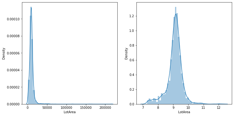
정규화(normalization)란 패턴 인식에서의 전처리의 일종으로 볼 수 있습니다.

좌측 그래프는 왼쪽으로 치우진 분포를 나타내고, 우측 그래프는 일반적인 가우시안 분포와 유사한 형태를 나타냅니다.

모델이 학습할 때, 특히 우리가 예측할 값(SalesPrice)에 대해서, 그리고 예측할 값과 선형관계인 수치형 column에 대하여 log를 취해줌으로써 보다 정교한 예측을 가능하게 합니다.

단, 주의해야할 점은 예측해야할 값인 (SalesPrice)에 대하여 log를 취해주었다면, 최종 값은 exp 메소드를 활용하여 원래 값으로 되돌려 놓는 작업이 필요합니다.

아래 예시를 통해 확인해보시죠.

# 150 이라는 숫자를 log로 변환
log_num = np.log(150)

log_num

5.0106352940962555

log_num을 다시 150으로 변환하려면 np.exp(log_num)으로 돌릴 수 있습니다.

# log_num을 원래 150으로 변환
np.exp(log_num)

149.99999999999997

하지만, 문제가 하나 있습니다.

x = np.linspace(0, 1.5, 10000)
y = np.log(x)
plt.plot(x, y)

[<matplotlib.lines.Line2D at 0x157cff8a7b8>]

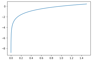
여기서 문제는 X 값이 0에 가까워지면 -무한대의 Y를 가지게 됩니다.

SalePrice 값이 만약 0이라면, log로 변환된 값은 -무한대의 값이 나와버려 오류가 생깁니다.

그래서 우리는 변환하기 전에 1을 더하여 변환시 -무한대의 값이 나오는 것을 방지할 수 있습니다.

바로 그 메소드가 np.log1p() 입니다.

# 150 이라는 숫자를 log로 변환
log_num = np.log1p(150)

log_num

5.017279836814924

되돌리기 위해서는 np.expm1()을 사용합니다.

# log_num을 원래 150으로 변환
np.expm1(log_num)

150.0

x = np.linspace(0, 1.5, 10000)
y = np.log1p(x)
plt.plot(x, y)

[<matplotlib.lines.Line2D at 0x157cfff79e8>]

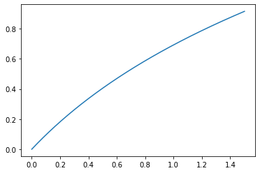
x = 0 일때, y의 최소값은 이제 0을 가지게 됩니다.

LotArea로 다시 돌아와서 정규화를 위한 log를 적용해 보도록 하겠습니다.

all_data['LotArea'] = np.log1p(all_data['LotArea'])

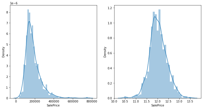
SalePrice도 분포를 살펴볼까요?

fig, axes = plt.subplots(1, 2)
fig.set_size_inches(12, 6)
sns.distplot(label, ax=axes[0])
sns.distplot(np.log1p(label), ax=axes[1])
plt.show()

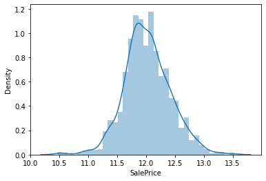
label = np.log1p(label)

sns.distplot(label)
plt.show()

필요없는 column 제거

다음 3개의 column에 대해서는 drop하여 사용하지 않겠습니다. 왜냐하면, 소수의 데이터를 제외한 대부분의 값들이 1개의 값으로 통일되기 때문에, 별다른 유의점이 없습니다. 오히려, 소수의 데이터가 모델의 성능을 떨어뜨릴 수 있습니다.

all_data['Utilities'].value_counts()

AllPub    2916
None         2
NoSeWa       1
Name: Utilities, dtype: int64

all_data['Street'].value_counts()

Pave    2907
Grvl      12
Name: Street, dtype: int64

all_data['PoolQC'].value_counts()

None    2909
Gd         4
Ex         4
Fa         2
Name: PoolQC, dtype: int64

remove_cols = [
    'Utilities',
    'Street',
    'PoolQC',
]

all_data = all_data.drop(remove_cols, 1)

print(all_data.shape)

(2919, 91)

cat_cols = all_data.select_dtypes(include = ["object"]).columns

print(len(cat_cols))

40

One Hot Encoding

카테고리 형 column에 대해서 one-hot-encoding을 적용합니다.

all_data = pd.get_dummies(all_data)

all_data.head()

	MSSubClass	LotFrontage	LotArea	OverallQual	OverallCond	YearBuilt	YearRemodAdd	MasVnrArea	BsmtFinSF1	BsmtFinSF2	...	SaleType_COD	SaleType_New	SaleType_Other	SaleType_WD	SaleCondition_Abnorml	SaleCondition_AdjLand	SaleCondition_Alloca	SaleCondition_Family	SaleCondition_Normal	SaleCondition_Partial
0	60	65.0	9.042040	7	5	2003	2003	196.0	706.0	0.0	...	0	0	0	1	0	0	0	0	1	0
1	20	80.0	9.169623	6	8	1976	1976	0.0	978.0	0.0	...	0	0	0	1	0	0	0	0	1	0
2	60	68.0	9.328212	7	5	2001	2002	162.0	486.0	0.0	...	0	0	0	1	0	0	0	0	1	0
3	70	60.0	9.164401	7	5	1915	1970	0.0	216.0	0.0	...	0	0	0	1	1	0	0	0	0	0
4	60	84.0	9.565284	8	5	2000	2000	350.0	655.0	0.0	...	0	0	0	1	0	0	0	0	1	0

5 rows × 279 columns

# 아래 코드는 바꾸지 마세요
# 총 279개의 column이 생성되어야 합니다.
assert len(all_data.columns) == 279
print(all_data.shape)

(2919, 279)

Train / Test 데이터 분리

all_data를 train / test로 다시 분리 합니다.

len(train), len(test)

(1460, 1459)

len(all_data[:len(train)]), len(all_data[len(train):])

(1460, 1459)

train_data = all_data[:len(train)]
test_data = all_data[len(train):]

# 코드를 변경하지 마세요
# 셀 실행시 에러가 나지 않아야 합니다.
assert len(train_data) == len(train)
assert len(test_data) == len(test)

앞선 단계에서 발견한 outlier를 제거합니다.

train_data = train_data.drop(outlier)
label = label.drop(outlier)

# 코드를 변경하지 마세요
# 셀 실행시 에러가 나지 않아야 합니다.
assert len(train_data) == len(train) - 2

평가 지표

from sklearn.metrics import mean_squared_error
from sklearn.model_selection import train_test_split

train_test_split 메소드를 활용하여 train set, validation set을 생성합니다.

비율은 train set = 80%, validation set = 20% 비율로 생성합니다.

train_test_split 사용 블로그 참고

Q11. x_train, x_valid, y_train, y_valid를 생성해 주세요

• x_train, y_train: train 데이터의 x, y
• x_valid, y_valid: valida 데이터의 x, y

len(train_data), len(label)

(1458, 1458)

# 이곳에 코드를 입력해 주세요
x_train, x_valid, y_train, y_valid = train_test_split(train_data, label, test_size=0.2, shuffle=True, random_state=34)

평가 지표 (MSE) 입니다. 아래 함수를 활용하여, 우리의 모델 성능을 가늠해 볼 수 있습니다.

# MSE 오차 평가
def get_score(y_pred, y_test):
    return np.sqrt(mean_squared_error(np.expm1(y_pred), np.expm1(y_test)))

모델링

아래 예시로, RidgeCV를 활용하여 가격 예측을 해봤습니다.

RidgeCV = Ridge 알고리즘에 Cross Validation 기능을 내제화한 모델입니다.

자세한 알고리즘 내용은 여기에서 확인하실 수 있습니다.

또한, 저는 RobustScaler라는 스케일러를 적용했는데, RubostScaler는 outlier를 제거함에 있어 좋은 스케일러입니다.

관련 내용은 여기에서 확인하실 수 있습니다.

아래 프로세스 대로 1개의 모델링과 평가지표를 활용하여 검증까지 진행합니다.

샘플로 제공되는 STEP처럼, 여러분들만의 단일 모델을 완성하고, 샘플 모델의 성능을 능가하는 모델을 만들어 보세요

STEP 1) 필요한 라이브러리 import

from sklearn.model_selection import KFold
from sklearn.preprocessing import RobustScaler
from sklearn.linear_model import RidgeCV
from sklearn.pipeline import make_pipeline

STEP 2) KFold (cross-validation) 체크를 위한 선언 (CV 모델을 사용하지 않으면, 굳이 필요없습니다.)

kf = KFold(random_state=30, 
           n_splits=10, 
           shuffle=True)

make_pipeline에 전처리 scaler와 model을 순차적으로 넣어주면, 알아서 scaler 적용 후 모델에 학습시킵니다.

STEP 3) 모델 선언, 하이퍼파라미터 설정

• pipeline을 만들어, scaler 적용 후 학습을 시킬 수 있습니다. 샘플로 보여드리기 위하여 가져온 코드이니, 여러분들은 꼭 이렇게 안해주어도 상관없습니다.

참고) RobustScaler는 outlier(이상치) 제거에 효과적인 스케일러 입니다.

# make pipeline
alphas_alt = [14.5, 14.6, 14.7, 14.8, 14.9, 15, 15.1, 15.2, 15.3, 15.4, 15.5]
ridgeCV = make_pipeline(RobustScaler(), RidgeCV(alphas=alphas_alt, cv=kf))

STEP 4) fit (학습)

# 학습
ridgeCV.fit(x_train, y_train)

Pipeline(steps=[('robustscaler', RobustScaler()),
                ('ridgecv',
                 RidgeCV(alphas=array([14.5, 14.6, 14.7, 14.8, 14.9, 15. , 15.1, 15.2, 15.3, 15.4, 15.5]),
                         cv=KFold(n_splits=10, random_state=30, shuffle=True)))])

STEP 5) predict (예측)

# validation 값에 대한 예측
valid_result = ridgeCV.predict(x_valid)

STEP 6) 평가지표를 활용하여, 모델의 성능 측정

# score 출력
get_score(valid_result, y_valid)

21489.69419660626

STEP 7) TEST 데이터에 대한 예측 후 특정 변수에 예측 값 저장

# test 값에 대한 예측
test_result = ridgeCV.predict(test_data)

여기서부터는 여러분들이 모델을 만듭니다.

여러분들의 모델을 만들어 최고의 성능을 발휘하는 모델을 완성합니다.

정답은 없습니다. 하지만, 목표 점수는 있습니다.

get_score() 기준으로 우선 19000 이하에 도전해 보세요

tip

• ensemble 모델은 5이상 만들어 보세요. 보통 ensemble 모델이 성능이 좋습니다.
• ensemble 모델끼리 ensemble을 적용해 보세요.
• weighted blending, stacking ensemble이 생소하다면, 검색을 통해 적용해 보세요

STEP 1) 필요한 라이브러리 import

# 코드를 입력해 주세요
from sklearn.linear_model import Lasso
from sklearn.linear_model import ElasticNet
from sklearn.pipeline import make_pipeline
from sklearn.preprocessing import StandardScaler
from sklearn.preprocessing import PolynomialFeatures
from sklearn.ensemble import GradientBoostingRegressor
from sklearn.ensemble import RandomForestRegressor
import lightgbm as lgb
import xgboost as xgb
from sklearn.ensemble import AdaBoostRegressor
from sklearn.ensemble import BaggingRegressor
from sklearn.ensemble import VotingRegressor

STEP 2) 모델 선언, 하이퍼파라미터 설정

lasso = Lasso(alpha=0.01)
lasso.fit(x_train, y_train)
lasso_pred = lasso.predict(x_valid)
get_score(lasso_pred, y_valid)

23651.46251664829

elasticnet = ElasticNet(alpha=0.01, l1_ratio=0.8)
elasticnet.fit(x_train, y_train)
eln_pred = elasticnet.predict(x_valid)
get_score(eln_pred, y_valid)

23107.90150308391

elasticnet_pipeline = make_pipeline(
    StandardScaler(),
    ElasticNet(alpha=0.01, l1_ratio=0.8)
)
elasticnet_pipeline.fit(x_train, y_train)
elasticnet_pred = elasticnet_pipeline.predict(x_valid)
get_score(elasticnet_pred, y_valid)

19573.98378665373

poly_pipeline = make_pipeline(
    PolynomialFeatures(degree=2, include_bias=False),
    ElasticNet(alpha=0.1, l1_ratio=0.2)
)
poly_pipeline.fit(x_train, y_train)
poly_pred = poly_pipeline.predict(x_valid)
get_score(poly_pred, y_valid)

20403981.644633118

gbr = GradientBoostingRegressor(random_state=30, learning_rate=0.01, n_estimators=1000, subsample=0.8)
gbr.fit(x_train, y_train)
gbr_pred = gbr.predict(x_valid)
get_score(gbr_pred, y_valid)

24965.372638372213

random_forest_model1 = RandomForestRegressor(n_estimators = 1000,
                                             max_depth = 7,
                                             max_features=0.9,
                                             random_state = 30)

random_forest_model1.fit(x_train, y_train)
rfr_pred = random_forest_model1.predict(x_valid)
get_score(rfr_pred, y_valid)

26900.348750434103

lgb_dtrain = lgb.Dataset(data = x_train, label = y_train) # 학습 데이터를 LightGBM 모델에 맞게 변환
lgb_param = {'max_depth': 10, # 트리 깊이
            'learning_rate': 0.01, # Step Size
            'n_estimators': 1000, # Number of trees, 트리 생성 개수
            'objective': 'regression'} # 목적 함수 (L2 Loss)
lgb_model = lgb.train(params = lgb_param, train_set = lgb_dtrain) # 학습 진행
lgb_pred = lgb_model.predict(x_valid) # 평가 데이터 예측
get_score(lgb_pred, y_valid)

27348.198902242944

xgb_model = xgb.XGBRegressor(n_estimators=1000, learning_rate=0.01, gamma=0, subsample=0.75, colsample_bytree=1, max_depth=10, random_state=30)
xgb_model.fit(x_train, y_train)
xgb_pred = xgb_model.predict(x_valid)
get_score(xgb_pred, y_valid)

[12:30:12] WARNING: src/objective/regression_obj.cu:152: reg:linear is now deprecated in favor of reg:squarederror.





26927.98689812403

Adaboost_model1 = AdaBoostRegressor( base_estimator = gbr,
                                     n_estimators = 100,
                                     random_state = 30) # 시드값 고정
Adaboost_model1.fit(x_train, y_train)
abr_pred = Adaboost_model1.predict(x_valid)
get_score(abr_pred, y_valid)

26549.717763738445

# Bagging
bag_model = BaggingRegressor(base_estimator=elasticnet_pipeline, n_estimators=100, random_state=30)

STEP 3) fit (학습)

#코드를 입력해 주세요
# Bagging
bag_model.fit(x_train, y_train)
bag_pred = bag_model.predict(x_valid)
get_score(bag_pred, y_valid)

19574.466197900896

# Voting
estimators = [
    # 앙상블 할 모델 정의
    ('bag', bag_model),
    ('elp', elasticnet_pipeline),
    ('pop', poly_pipeline),
    ('RidgeCV', ridgeCV),
    ('eln', elasticnet)
]

weights=[5, 5, 1, 1, 1]
vr_model1 = VotingRegressor(estimators, weights)
vr_model1.fit(x_train, y_train)
vr_pred = vr_model1.predict(x_valid)
get_score(vr_pred, y_valid)

21644.634424352244

# Stacking 앙상블
estimators = [
    # 앙상블 할 모델 정의
    ('rcv', ridgeCV),
    ('las', lasso),
    ('eln', elasticnet),
    ('elp', elasticnet_pipeline),
    ('pop', poly_pipeline),
    ('gbr', gbr),
    ('raf', random_forest_model1),
    ('xgb', xgb_model),
    ('ada', Adaboost_model1),
    ('bag', bag_model)
]

from sklearn.ensemble import StackingRegressor
str_model = StackingRegressor(
    estimators=estimators,
    final_estimator=bag_model, n_jobs=-1)
str_model.fit(x_train, y_train)
str_pred = str_model.predict(x_valid)
get_score(str_pred, y_valid)

20224.106063727144

STEP 4) predict (예측) - x_valid 에 대한 예측

#코드를 입력해 주세요

# Weighted Blending
blend = elasticnet_pred * 0.4 + bag_pred * 0.3 + poly_pred * 0.1 + valid_result * 0.1

STEP 5) 평가지표를 활용한 성능 측정

#코드를 입력해 주세요
# Bagging 성능
get_score(bag_pred, y_valid)

19574.466197900896

#코드를 입력해 주세요
# Weighted Blending 성능
# 궁금증이 있습니다. Weighted Blending 은 단순 평가 지표 (MSE)를 받기 위해 사용 되는건가요?
get_score(blend, y_valid)

146103.24601337546

STEP 6) predict (예측) - test_data 에 대한 예측

test_result = bag_model.predict(test_data) 

# 이곳에 코드를 입력해 주세요
final_result = blend

# 코드를 변경하지 마세요
print(final_result[:5])
print()
print('최종 점수: {:.3f}'.format(get_score(final_result, y_valid)))

[10.47151862 10.34366343 10.60970687 10.20004478 10.53560791]

최종 점수: 146103.246

final_prediction에는 test data를 기준으로 예측한 값을 대입해 줍니다.

# 최종 예측 값
final_prediction = test_result

# 검증코드
assert final_prediction.shape[0] == 1459

Kaggle 에 제출하기

먼저, submission파일에 우리가 예측한 정답 값을 입력하겠습니다.

from datetime import datetime

t = datetime.now().strftime('%Y-%m-%d-%H-%M')
filename = '{0}-submission.csv'.format(t)
# 파일 이름을 확인합니다.
print(filename)

2020-12-04-13-18-submission.csv

sample_submission = pd.read_csv('https://bit.ly/fc-ml-byte-submission')

예측한 값을 다시 np.expm1()을 통해 역스케일 합니다.

final_prediction = np.expm1(final_prediction)

.csv파일로 최종 저장하고 결과를 제출하여 점수를 확인합니다.

sample_submission['SalePrice'] = final_prediction
sample_submission.to_csv(filename, index=False)

Extra. Kaggle 상위권에 도전하기

상위 20% 안에 든다면, Data Scientists로써 인정받을 수 있는 점수 입니다.

Kaggle은 글로벌 Data Scientists, Machine Learning 엔지니어들이 다양한 데이터 분석 기법과 머신러닝 스킬을 총동원하여 최고의 예측을 할 수 있도록 겨루는 공간입니다.

여러분들이 만약 상위 20% 안에 드는 점수를 기록한다면, 프로필에도 상위 20% 점수를 획득했다고 공개됩니다.

여러분들의 순수 업적으로 기록 될 수 있습니다. 최고에 한 번 도전해 보세요!

캐글에 제출하여 점수 확인하기: House Prices

• 위의 링크를 클릭하여, 우리가 생성한 submission 파일을 제출하고, 점수를 확인합니다.
• 리더보드에서 내가 획득한 점수가 몇등인지 확인할 수 있으며, 더 높은 곳을 향해 도전합니다.